Make Better Team Decisions: 4 Steps Using Bayesian Updating

Bayesian updating is the process of revising a probability for a hypothesis using Bayes’ theorem: posterior probability is proportional to likelihood times prior. It gives you a disciplined way to fold new evidence into what you already believed, rather than throwing out old beliefs or ignoring new data. You use it whenever you need to reason under uncertainty and update as evidence arrives, from diagnosing a disease to deciding whether a product experiment actually worked.

---

TL;DR:

• Beliefs are highly sensitive to prior assumptions, so choosing weakly informative priors helps maintain robustness as new evidence accumulates.
• Bayesian updating is most effective in sequential, small-sample, or high-stakes decision contexts where calibration and prior knowledge are crucial.
• Conjugate priors simplify calculations and allow for direct parameter updates, making real-time updates feasible without complex numerical methods.
• Numerical methods like MCMC and variational inference are necessary only for complex models lacking closed-form solutions, but diagnostics are essential for reliable results.
• Teams should adopt a habit of recording initial beliefs, updating with incoming evidence, and documenting outcomes to improve calibration and decision quality over time.

---

What Is Bayesian Updating, Really?

Being “Bayesian” means treating a belief as a number between 0 and 1, and being willing to move that number when you see new evidence. That is the whole idea. Most people already think this way informally. If your friend is usually on time but texts “running late,” you do not conclude she will never arrive. You just lower your confidence that she’ll be there at 7:00 sharp. Bayesian updating just makes that intuition mathematically precise.

Four pieces make up the machine:

• Prior: your probability estimate for a hypothesis before seeing the new evidence.
• Likelihood: how probable the observed evidence is, assuming a specific hypothesis is true.
• Posterior: your updated probability estimate for the hypothesis after accounting for the evidence.
• Marginal likelihood: the overall probability of the evidence, averaged across every hypothesis you’re considering. It acts as a normalizing constant so all your posterior probabilities still sum to 1.

Here’s a classic example that shows why this matters. Suppose a disease is rare, and a test for it has high accuracy for both true positives and true negatives. If you test positive, your initial feeling might be that you’re almost certainly sick. Bayesian math says otherwise: because the disease is uncommon, false positives from the healthy population can outnumber true positives from the sick, and your actual probability of having the disease will be much lower than the test accuracy alone might suggest. That gap between intuition and the correct answer is exactly why thinking probabilistically instead of in absolutes changes how good your decisions are. Teams that get comfortable with intervals and updated confidence, rather than binary yes/no calls, tend to catch these traps before they cost anything.

The coin toss version is simpler and worth keeping in your back pocket. If you’re not sure whether a coin is fair, your prior might put 50% odds on “fair” and split the rest across biased possibilities. Every flip you observe is evidence. Ten heads in a row does not prove the coin is rigged, but it should shift your posterior hard toward “probably biased,” and Bayesian updating tells you exactly how hard.

Bayesian updating earns its keep in a specific set of situations:

• Sequential decisions, where evidence trickles in over time instead of arriving all at once (clinical trials, A/B tests, fraud detection).
• Small-sample problems, where you need a sensible answer before you have a lot of data.
• Situations demanding calibrated confidence, not just a point estimate, like weather forecasting or credit risk models.
• Any decision where prior knowledge is genuinely informative and throwing it away would waste real information.

How Does Bayes’ Theorem Actually Work?

Bayes’ theorem states: P(H|D) = P(D|H) × P(H) / P(D). In plain language, the probability of a hypothesis given the data equals the probability of the data given the hypothesis, times the prior probability of the hypothesis, divided by the overall probability of the data. Most practitioners drop the denominator when working through a problem and just write posterior ∝ likelihood × prior, then normalize at the end. That proportional form is how Bayesian inference gets used in practice, and it’s worth memorizing before you memorize the formal version.

The derivation is only a few lines, and walking through it once removes any sense that Bayes’ theorem is magic. It comes straight from the definition of conditional probability.

1. Conditional probability defines P(H|D) = P(H and D) / P(D), and by the same logic, P(D|H) = P(H and D) / P(H).
2. Both expressions share the same numerator, P(H and D), so you can set P(H|D) × P(D) equal to P(D|H) × P(H).
3. Divide both sides by P(D) and you get Bayes’ theorem: P(H|D) = P(D|H) × P(H) / P(D).
4. To compute P(D), the marginal likelihood, apply the law of total probability: sum P(D|H_i) × P(H_i) across every hypothesis H_i you’re considering. If there are three candidate hypotheses, you calculate three numerators, add them up, and that sum becomes your denominator.

Notation trips people up more than the math does. H stands for the hypothesis you care about, whether that’s “this coin is fair,” “this patient has the disease,” or “this marketing channel is driving the lift.” D stands for the data or evidence you just observed. P(H) is your prior. P(D|H) is the likelihood, which answers “if this hypothesis were true, how likely is this exact evidence?” P(H|D) is the posterior, the number you actually want.

The marginal likelihood, P(D), deserves special attention because it’s the part most people find counterintuitive. It is not the probability of the hypothesis. It is the probability of seeing that specific piece of evidence at all, averaged over every hypothesis in your model. It functions purely as a normalizing constant, forcing all your posterior probabilities to add up to 1 across a discrete set of hypotheses, or to integrate to 1 across a continuous parameter. One insight that saves a lot of arithmetic: when you’re only comparing hypotheses against each other, you often don’t need to compute P(D) explicitly at all. You can work with the unnormalized numerators, prior times likelihood, and only normalize at the very end once you’ve added everything up.

There’s a related concept worth knowing before you get to the worked examples: the posterior predictive distribution. Once you have a posterior over your hypothesis or parameter, you can ask a follow-up question: given everything I now believe, what’s the probability of the next observation? That’s the posterior predictive distribution, and it’s what you actually use to make forward-looking predictions rather than just describing past evidence. In a medical testing context, it’s the difference between “how confident am I this patient has the disease” and “how likely is the next test to also come back positive.”

One clarification that heads off a lot of confusion: Bayes’ theorem itself is just algebra, uncontroversial and provable from the axioms of probability. What’s philosophically interesting, and where debates with frequentist statistics start, is the interpretation of P(H) as a genuine degree of belief rather than a long-run frequency. Keep that distinction in mind. The math is not in dispute. The interpretation is what makes Bayesian statistics methods a distinct school of thought.

What Does a Bayesian Update Table Look Like?

A Bayesian update table is the clearest way to see exactly how prior beliefs turn into posterior beliefs, one row of arithmetic at a time. Set one up, work through it by hand once, and you’ll never find the theorem abstract again.

Imagine you’re handed one of three coins pulled from a bag, and you don’t know which. Coin A is fair. Coin B is biased toward heads. Coin C is biased toward tails. Your prior, before any flips, is that each coin was equally likely to be drawn:

• Hypotheses and priors: The prior probabilities for hypotheses A, B, and C differ but are not perfectly even, reflecting more fair coins than biased ones.
• Likelihoods: Each coin has a characteristic probability of producing heads, with one fair coin and biased versions favoring heads or tails.

You flip the coin once and get heads. Here’s the table:

The mechanics, laid out step by step, following the same approach used in MIT’s course notes on Bayesian updating:

• Multiply each hypothesis’s prior by its likelihood to get an unnormalized numerator.
• Add up all three numerators to get P(D), the marginal likelihood: 0.4875 in this case.
• Divide each numerator by that total to get the posterior for each hypothesis.
• Confirm the posteriors sum to 1.000, which they do here, as a sanity check on your arithmetic.

One flip of heads already moved your belief. Coin A barely moved, because a fair coin producing heads is unremarkable evidence either way.

The real value shows up when you flip again. Your posterior from the first flip becomes your prior for the second. Flip heads again, and you’d multiply this new prior column by the same likelihoods, form new numerators, and renormalize. There’s a computational shortcut worth knowing here: when you’re chaining several observations together, you don’t have to normalize after every single flip. You can multiply the raw numerators across all observations first and normalize only once at the end, which saves work when you’re tracking a long sequence of evidence rather than updating one flip at a time.

Run three tails in a row and Coin C dominates instead. This is where probabilistic decision making gets practical: if you needed to decide, after five flips, whether to bet money on which coin you’re holding, the posterior distribution tells you exactly how confident you should be, and at what point the evidence clears a reasonable decision threshold. A posterior of 53% is not a strong enough signal to act on.

What Are Conjugate Priors and Why Do They Matter?

A conjugate prior is a prior distribution that, when combined with a particular likelihood, produces a posterior in the exact same distributional family. That property turns Bayesian updating from a numerical table exercise into simple arithmetic on a couple of parameters, which is why conjugate priors show up in nearly every introductory course on Bayesian statistics methods.

The most common example is the Beta-Binomial pair, used whenever you’re estimating a probability from binary outcomes, success or failure, click or no click, converted or not converted.

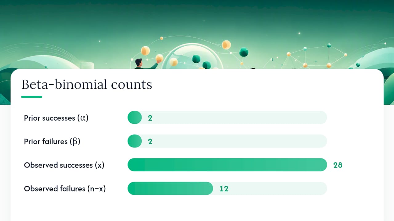
1. Start with a Beta(α, β) prior over the unknown probability p. Think of α as your prior count of successes and β as your prior count of failures, whether or not you observed them directly. A Beta(2, 2) prior is mildly skeptical and centered at 50%; a Beta(1, 1) prior is flat and uninformative.
2. Observe data: x successes out of n trials.
3. The posterior is simply Beta(α + x, β + n − x). No integration, no numerator table, no normalizing sum required.
4. To get a point estimate, use the posterior mean: (α + x) / (α + β + n).

You run 40 visitors through and get 28 conversions. Every additional visitor updates those two numbers directly. No table required.

The Normal-Normal case handles continuous measurements: estimating a mean when the data itself is roughly bell-shaped, like average order value, response time, or a sensor reading with known measurement noise.

1. Assume the data has known variance σ², and your prior belief about the true mean μ is Normal(μ₀, σ₀²).
2. After observing n data points with sample mean x̄, the posterior is also normal, with a new mean and a new, smaller variance.
3. The posterior mean is a weighted average of your prior mean and the observed sample mean, where the weights are the precisions (inverse variances) of each source.
4. The posterior variance shrinks as more data arrives, since precision is additive: posterior precision equals prior precision plus data precision.

That weighting is the intuition worth holding onto: your prior behaves as if it contributes its own “effective sample size” worth of data, competing against the actual observed sample size. A strong, tight prior (equivalent to hundreds of hypothetical observations) barely budges when you feed it 10 real data points. A weak, diffuse prior gets steamrolled by even a modest amount of real data. Neither behavior is wrong. It’s exactly what should happen when you think about priors as accumulated evidence rather than arbitrary guesses.

This is also why conjugate models are so useful for teaching and for real-time systems: updating is just addition. A recommendation engine tracking click-through rate per item, or a call center tracking average handle time, can update its Beta or Normal parameters after every single new data point without touching a table or running a solver.

How Do You Compute a Bayesian Update Without a Closed Form?

Most real-world models don’t have a tidy conjugate solution, and that’s when you switch to numerical methods: Markov Chain Monte Carlo (MCMC), importance sampling, or variational inference. Each earns its place under different conditions, and MIT’s OpenCourseWare materials on Bayesian methods treat these as the standard toolkit once a problem moves past textbook conjugacy.

MCMC methods, including the Metropolis-Hastings algorithm and Hamiltonian Monte Carlo, work by drawing a long sequence of correlated samples that eventually approximates your true posterior distribution. Use MCMC when your parameter space is moderate in size and you care more about getting an accurate posterior than about speed. Importance sampling reweights samples drawn from an easier distribution to approximate a harder one, and it works well when you already have a reasonable proposal distribution close to the true posterior. Variational inference turns the whole problem into an optimization task, approximating the posterior with a simpler distribution and fitting it fast. Reach for variational methods when your dataset or parameter space is large and you need speed over exactness, which is common in modern machine learning pipelines.

None of these methods are trustworthy without diagnostics. Before you believe any posterior estimate that came out of MCMC, check the following:

• Run multiple chains starting from different initial values and confirm they converge to the same distribution.
• Check R-hat, the potential scale reduction factor; values close to 1.0 indicate the chains agree with each other.
• Check effective sample size (ESS), since correlated MCMC samples carry less information than the same number of independent draws would.
• Look at traceplots visually. A healthy chain looks like noise bouncing around a stable band. A chain that drifts or gets stuck signals a real problem.
• Run posterior predictive checks: simulate new data from your fitted posterior and compare it to the data you actually observed. Systematic mismatches are a warning that your model is misspecified, not that your data is strange.

A simple online update loop, in outline form, looks like this: maintain a current posterior (or its sufficient statistics, if you’re in a conjugate case); when a new observation arrives, treat the current posterior as the new prior; multiply by the likelihood of the new data point; renormalize (or, in the conjugate case, just update the parameters directly); store the new posterior; repeat.

Pro Tip: When you’re implementing any of this in code, work in log-probabilities instead of raw probabilities. Multiplying many small probability values together underflows to zero shockingly fast on real hardware. Adding log-likelihoods keeps your numbers stable and is the standard practice in almost every serious probabilistic programming library.

Where Does Bayesian Updating Actually Get Used?

Bayesian updating shows up anywhere evidence arrives in pieces and a decision can’t wait for perfect certainty. Four domains use it constantly:

• Machine learning and AI, where model parameters get updated as new training data or feedback arrives, and where probabilistic reasoning underlies everything from spam filters to recommendation systems and Bayesian network analysis.
• Clinical diagnostics, where a doctor’s pretest probability, based on symptoms and prevalence, gets revised by each new test result rather than treated as a single, final verdict.
• Forecasting, where weather models and election forecasters continuously update probability estimates as new data streams in, rather than issuing one static prediction and waiting.
• Reliability engineering, where failure-rate estimates for equipment get refined as more usage data and failure events accumulate over a product’s life.

The common thread across all four is that Bayesian updating rewards evidence incorporation over time instead of demanding one big dataset upfront. That’s a genuinely different mode of thinking than a lot of statistical training, which tends to assume you collect everything first and analyze once. Real decisions rarely work that way. Evidence dribbles in, and the model needs to move with it.

There’s a decision-quality angle here too, and it matters as much for teams as it does for models. Calibrated confidence, meaning your stated probability actually matches your long-run accuracy, is what separates a useful forecast from a confident guess. Teams that get in the habit of writing down a probability before an outcome is known, and then checking how that probability compares to what actually happened, tend to get better at judgment over time. That’s the same discipline decision education researchers point to when they argue that admitting uncertainty upfront, instead of defaulting to false confidence, produces better outcomes on average.

This is where Bayesian thinking stops being a math exercise and becomes an organizational habit. A team that documents a hypothesis, assigns it a confidence level, gathers evidence, and then records how that confidence shifted is running an informal Bayesian update every time it makes a real decision. A structured decision journal is one practical way to make that loop explicit: log the prior belief and the reasoning behind it, log the evidence as it comes in, and log the posterior once a decision gets made, so nothing gets lost between the guess and the outcome.

What Goes Wrong When People Misuse Bayesian Updating?

The single biggest failure mode is prior sensitivity: a poorly chosen prior can dominate a posterior when data is scarce, and two analysts working the same problem with different priors can land on very different conclusions. This isn’t a flaw in the math. It’s a feature that demands honesty about where your prior actually came from.

A short list of the mistakes that show up most often in practice:

• Overconfident priors: setting a prior so narrow (a Beta(200, 200), for instance, instead of a Beta(2, 2)) that no realistic amount of new data can move it.
• Ignoring model mismatch: a posterior can look perfectly clean and still be wrong if the underlying likelihood function doesn’t match how the data was actually generated.
• Data dredging: peeking at results repeatedly and stopping the moment the posterior looks favorable, which quietly injects bias into what should be an honest sequential update.
• Treating the posterior as certainty: a 90% posterior probability is still a probability, not a guarantee, and decisions should reflect that gap.

Running a sensitivity analysis is the standard defense: refit the same model with two or three meaningfully different priors, from skeptical to permissive, and see whether your conclusion holds up across all of them. If your answer flips depending on which reasonable prior you picked, you don’t have a robust conclusion yet, no matter how clean the posterior distribution looks. Bayesian inference is not the only rule for updating beliefs under uncertainty, either. Jeffrey’s rule and probability kinematics offer alternative approaches, built for situations where the new evidence itself is uncertain rather than a clean, observed fact.

Practitioners are generally advised to use probabilistic intervals rather than absolute point estimates when tracking beliefs over time, specifically to guard against overconfidence in team decisions, according to the Alliance for Decision Education.

Practical mitigations worth adopting as habits rather than one-off fixes: default to weakly informative priors unless you have a specific, defensible reason to be more confident; hold out data for cross-validation rather than fitting and evaluating on the same set; and run posterior predictive checks before trusting a model’s output in a live decision.

How Should Teams Actually Use Bayesian Updating Day to Day?

Most teams don’t need MCMC or a conjugate derivation to benefit from Bayesian thinking. They need a habit: write down what you believe and how confident you are, before you act, and check it against what actually happened.

A workable version of that habit runs in four steps:

• State the hypothesis and prior confidence. Write the belief in plain language (“this pricing change will lift conversion”) and attach an honest number to it, even a rough one like 60%.
• Log the evidence as it arrives. Record the data point, the experiment result, or the customer feedback that’s relevant, as soon as it shows up, before hindsight has a chance to distort it.
• Update the belief, formally or informally. Sometimes that’s a real Beta-Binomial calculation. More often, for a business decision, it’s an honest gut recalibration: “I was at 60%, this new data pushes me to 80%.”
• Record the decision and the eventual outcome separately. The decision and the outcome are not the same thing, and conflating them is exactly how organizations lose the ability to tell a good process from a lucky result.

The payoff isn’t philosophical. It’s that reasoning survives past the moment it was written down. Most teams lose their best thinking the day after a decision gets made, because nobody wrote why they believed what they believed, or how confident they actually were. A structured record turns every decision into a small experiment with a documented hypothesis, instead of a one-off judgment call that vanishes into the general memory of “how things went.”

That is the specific gap Betlog was built to close: a decision journal that captures the hypothesis, the confidence level, and the trade-offs before a commitment gets made, then keeps that record permanently so a team can look back and see whether its confidence was calibrated, not just whether the outcome was good. Judging decisions purely by outcomes throws away exactly the information a Bayesian update depends on: what you believed, and why, before you knew how things turned out.

Where Can You Learn More About Bayesian Methods?

If you want to go deeper than this article, the reading list depends on where you’re starting.

Beginners should start with the Bayesian inference overview on Wikipedia, which lays out the formal structure, terminology, and historical context in a format you can revisit as a reference. From there, accessible tutorials like Towards Data Science’s walkthrough of Bayesian updating bridge the gap between the formula and working code, which is often the hardest jump for self-taught learners.

For a more rigorous, course-style treatment, MIT’s class notes on Bayesian updating walk through the discrete update table mechanics in detail, and the companion MIT OpenCourseWare reading on Bayes and probability covers the numerical methods, MCMC diagnostics, and implementation notes that this article only summarizes. Advanced readers chasing conjugate derivations and hierarchical models should treat those two documents as a starting syllabus, not a finish line.

The Editorial Take: Start Simple, Then Scale the Math

The conventional advice on Bayesian updating oversells the math and undersells the habit. Plenty of guides jump straight to conjugate priors and MCMC diagnostics as if the formula is the hard part. It isn’t. The hard part is admitting, honestly, what you believed before you saw the evidence, and writing that number down where you can’t quietly revise it later.

Most of the value in Bayesian thinking shows up before you touch a posterior calculation: stating a real prior, resisting the urge to round it up to “obviously true” after the fact, and separating the quality of your reasoning from the luck of the outcome. The math matters for anyone doing serious modeling work, and conjugate priors and MCMC are worth learning properly. But for a founder or a small team trying to make better calls, the discrete update table taught here does more good than a variational inference tutorial ever will, because it’s the version you can actually run in your head during a Monday planning meeting.

Prioritize the habit first. Add the math when a specific decision actually demands precision.

— Phil

Sources

• Bayesian inference — Wikipedia
• Thinking probabilistically — Alliance for Decision Education
• Bayesian updating — MIT course notes

FAQ

What Does It Mean to Be Bayesian?

Being Bayesian means treating probability as a personal degree of belief that you revise as new evidence arrives, rather than as a fixed frequency you calculate once and leave unchanged.

What Does It Mean to Update Priors?

Updating a prior means combining your existing belief about a hypothesis with new evidence, using Bayes’ theorem, to produce a posterior probability that reflects both what you believed before and what you just observed.

Can You Explain Bayesian Inference in a Simple Way?

Bayesian inference starts with a prior probability, multiplies it by how likely the new evidence would be under each hypothesis, and normalizes the result so the updated probabilities, called posteriors, still add up to 1.

Why Does the Order of Evidence Not Matter in Bayesian Updating?

Because each update multiplies numerators together before normalizing, the same set of observations produces the same posterior regardless of the order they arrive in, as long as you process all of them.

What Is the Difference Between Bayesian and Frequentist Updating?

Frequentist methods treat probability as a long-run frequency and generally don’t formally incorporate prior beliefs into a calculation, while Bayesian updating explicitly combines a prior with new data through Bayes’ theorem to produce a posterior belief.